Saibaba At The Base Of A Banyan Tree In A Street
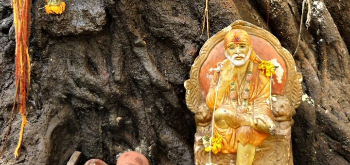
Saibaba worshipped on a busy street at the base of a banyan tree. Sai Baba is worshipped by people around the world. He had no love for perishable things and his sole concern was...
Saibaba worshipped on a busy street at the base of a banyan tree. Sai Baba is worshipped by people around the world. He had no love for perishable things and his sole concern was...
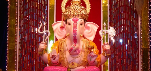
The most popular story as to how Ganapati lost his tusk is as follows. Veda Vyasa decided to compose the huge epic Mahabharata. He needed some body to write down his composition, as soon...

Tissot Watch Tissot is a luxury Swiss watchmaking company founded in Le Locle, Switzerland by Charles-Félicien Tissot and his son Charles-Émile Tissot in 1853. Tissot introduced the first mass-produced pocket watch as well as...
Qatar Qatar, officially the State of Qatar, is a sovereign Arab country located in Southwest Asia, occupying the small Qatar Peninsula on the northeastern coast of the Arabian Peninsula. Its sole land border is...

Nail Polish Nail polish is a lacquer that can be applied to the human fingernails or toenails to decorate and protect the nail plates. The formulation has been revised repeatedly to enhance its decorative...

Norway Norway, officially the Kingdom of Norway, is a sovereign and unitary monarchy whose territory comprises the western portion of the Scandinavian Peninsula plus Jan Mayen and the Arctic archipelago of Svalbard. The Antarctic...

Omega SA Omega Swatch LCD shows the time. Various models in different colors of the LCD are available which include back lighting for reading in the dark. Omega SASA is a Swiss luxury watchmaker...

Common Nightingale The common nightingale or simply nightingale also known as rufous nightingale is a small passerine bird best known for its powerful and beautiful song. Its song is particularly noticeable at night because...

Google Search Google Search, commonly referred to as Google Web Search or just Google. It is a web search engine owned by Google Inc. It is the most-used search engine on the World Wide...

Gucci Gucci is an Italian fashion and leather goods brand, part of the Gucci Group, which is owned by the French company Kering, formerly known as PPR. Gucci was founded by Guccio Gucci in...

Maltese The Maltese is a small breed of dog in the Toy Group. Characteristics include slightly rounded skulls with a finger-wide dome, a black button nose and brown eyes. The body is compact with...

432 Park Avenue, New York City 432 Park Avenue is a supertall residential project with 104 condominium apartments developed by CIM Group in midtown Manhattan, New York City. At a height of 425.5 m,...

Mahatma Gandhi Mohandas Karamchand Gandhi (2 October 1869 – 30 January 1948) was the preeminent leader of the Indian independence movement in British-ruled India. Gandhi led India to independence and inspired movements for civil...
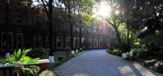
The Doon School, Uttarakhand The Doon School is a boys-only independent boarding school in Dehradun, India. It was founded in 1935 by Satish Ranjan Das, a Kolkata lawyer. The school is a member of...

Cricket Cricket is a bat-and-ball game played between two teams of 11 players each on a field at the center of which is a rectangular 22-yard long pitch. The game is played by 120...
Antarctic fur seal The Antarctic fur seal is one of eight seals in the genus Arctocephalus and one of nine fur seals in the subfamily Arctocephalinae. This fur seal is a fairly large animal...
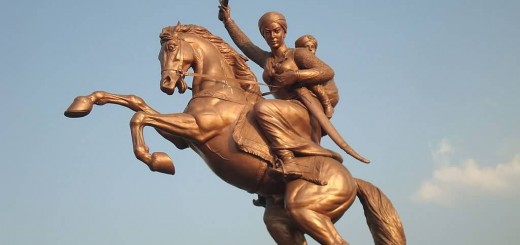
Rani Lakshmi Bai Lakshmibai, the Rani of Jhansi (19 November 1828 – 17/18 June 1858) was an Indian queen and warrior. She was one of the leaders of the Indian Rebellion of 1857 and...
Polar Bear The polar bear is a carnivorous bear whose native range lies largely within the Arctic Circle encompassing the Arctic Ocean its surrounding seas and surrounding land masses. The polar bear is a...
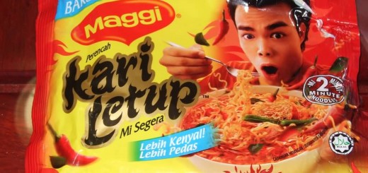
Maggi Maggi is an international brand of seasonings, instant soups and noodles owned by Nestle since 1947. The original company came into existence in 1875 in Switzerland, when Julius Maggi took over his father’s...

Chiang Rai Chiang Rai is the northernmost province of Thailand. It is bordered by the Shan State of Myanmar to the north, Bokeo Province of Laos to the east, Phayao to the south, Lampang...
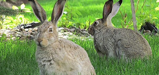
Angora Wool Angora wool or Angora fiber refers to the down coat produced by the Angora rabbit. There are many types of Angora rabbits – English, French, German and Giant. Angora is prized for...